UniOviSOM toolbox

Basic example

In this basic example we shall demonstrate the basic usage of uniovisom, including training a 20x20 SOM, plotting data and SOM in the input and the visualization space as well as showing the component planes, the distance map (u-matrix) and and the activation maps.

Define a basic dataset

Generate a basic training set in the input space to play with. In this case we consider 3D data points (n=3) to show also the SOM and the data in the input space

p = [randn(3,100)-5 randn(3,100)+5 randn(3,200)+[1;0;0]*ones(1,200)];

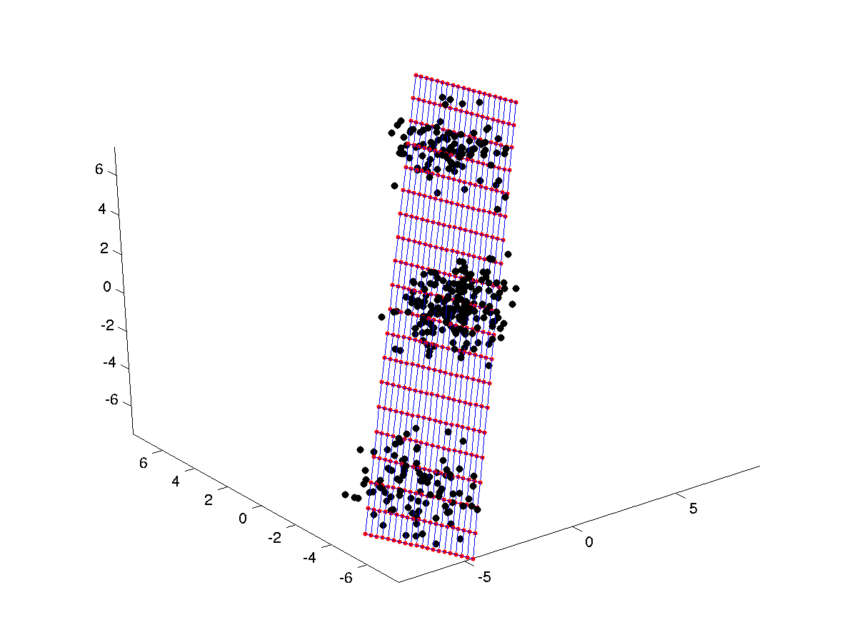
Plot the training set (if the input data hade more than 3 dimensions, uniovisom only shows the first three dimensions)

figure(1);
plotp(p);

Train and visualize a SOM model

Initialize a 2-D SOM with a rectangular topology of 20 by 20 codebook vectors

som = inisom(p,{20,20});

Plot the initialized SOM along with the input data

figure(2);
plotsom(p,som);

as seen, the SOM codebooks are initialized using a 2D PCA projection. Now, let's train the SOM with the data. Let uniovisom choose number of epochs and neighbourhood

som = bsom(p,som);      

Plot the trained SOM along with the input data set

figure(3);
plotsom(p,som);

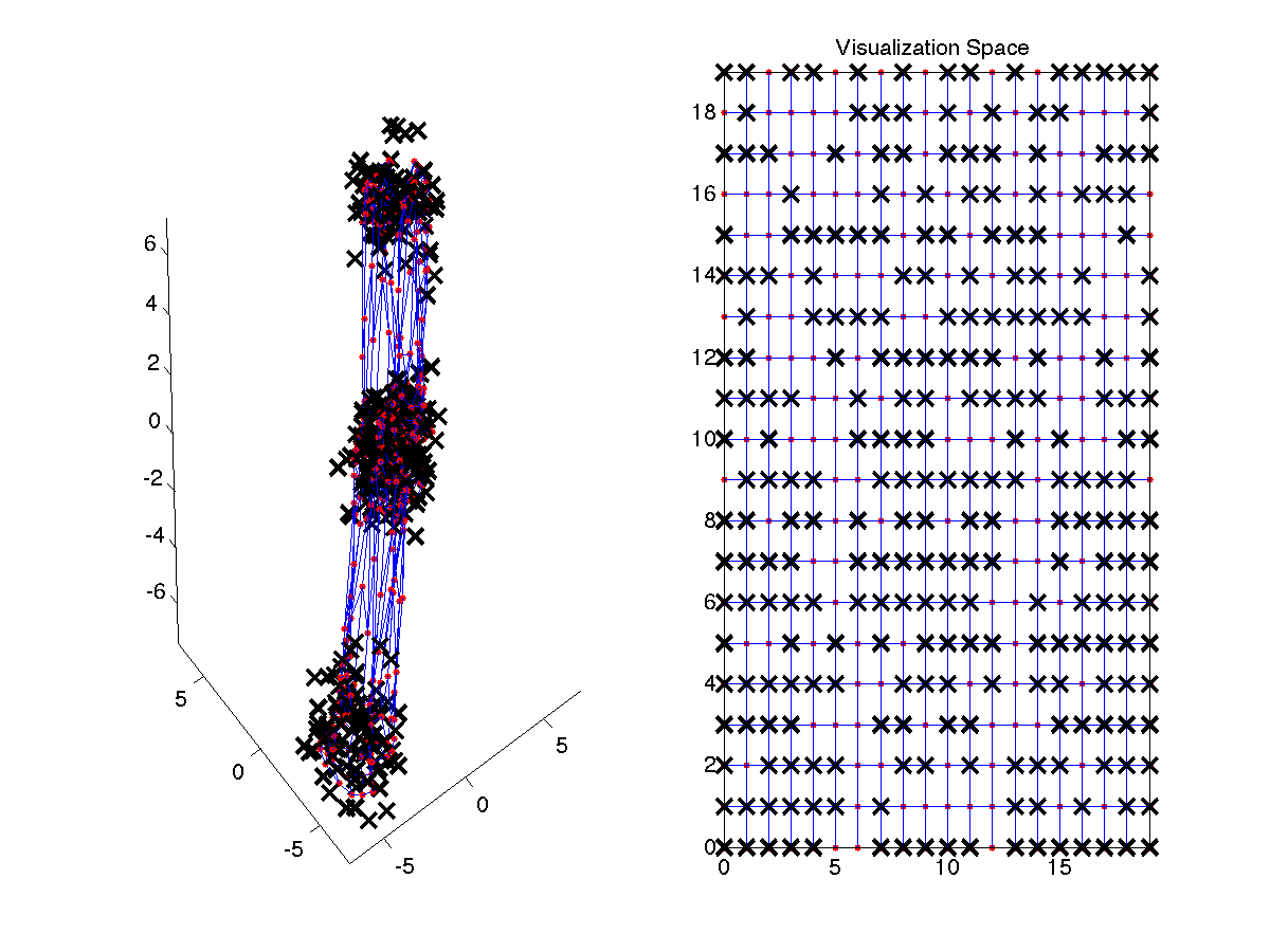
Plot the SOM and the data in the input and output space

figure(4);
plotsom(p,som,'both');

Plot the SOM component planes

figure(5);
planes(som);

Plot the distance map and the activation map of the first cloud of data. The distance map allows you to visualize in the 2D visualization space, the clusters from the input data space. The activation map shows you the region of the visualization space activated by given subset of n-dim data

figure(6);
dist = somdist(som);
actv = activation(p(:,1:100),som);
planes(som.pos,[dist;actv],{'Distance Map','Activation Map'});

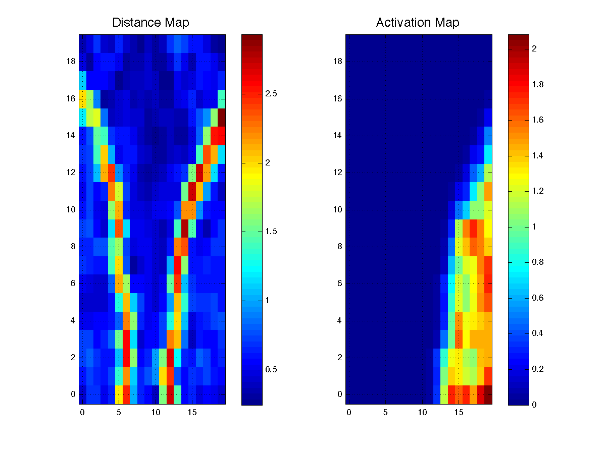we can see that the distance map, reveals three regions by showing their borders, whole the activation map, shows the region corresponding to the first 100 data points from our input dataset.

% Demo001 A SIMPLE EXAMPLE OF SOM TRAINING
%
% This example includes the following features:
%   - Generation of a training data set
%   - Initialization and training of a 2D SOM object
%   - Visualization of the input and output space
%   - Visualization of the SOM planes
%   - Computation of the SOM interneuron distance map
%   - Computation of the activation map generated by a labelled data set
%   - Visualization of the previous distance and activation maps

%   Copyright (c) 2007, by 
%   Grupo de Supervisión y Diagnóstico de Procesos Industriales
%   Area de Ingeniería de Sistemas y Automática
%   Universidad de Oviedo
%   Contributed files may contain copyrights of their own.
%   
%   UniOviSOM toolbox is free software; you can redistribute it and/or modify
%   it under the terms of the GNU General Public License as published by
%   the Free Software Foundation; either version 2 of the License, or
%   (at your option) any later version.
% 
%   This program is distributed in the hope that it will be useful,
%   but WITHOUT ANY WARRANTY; without even the implied warranty of
%   MERCHANTABILITY or FITNESS FOR A PARTICULAR PURPOSE.  See the
%   GNU General Public License for more details.
% 
%   You should have received a copy of the GNU General Public License
%   along with this program; if not, write to the Free Software
%   Foundation, Inc., 675 Mass Ave, Cambridge, MA 02139, USA.


% Generate a training set of data points in the input space
p = [randn(3,100)-5 randn(3,100)+5 randn(3,200)+[1;0;0]*ones(1,200)];

% Plot the training set
figure(1);
plotp(p);

% Initialize a 2-D SOM object
som = inisom(p,{20,20});

% Plot the initiazlized SOM along with the input data
figure(2);
plotsom(p,som);

% Train the SOM with the data
som = bsom(p,som);      % Let uniovisom choose number of epochs and neighbourhood

% Plot the trained SOM
figure(3);
plotsom(p,som);

% Plot the SOM and the data in the input and output space
figure(4);
plotsom(p,som,'both');

% Plot the SOM planes
figure(5);
planes(som);

% Plot the distance map and the activation map of the first cloud of data
figure(6);
dist = somdist(som);
actv = activation(p(:,1:100),som);
planes(som.pos,[dist;actv],{'Distance Map','Activation Map'});