% Demo002 A 3D SOM example


%   Copyright (c) 2007, by
%   Grupo de Supervisión y Diagnóstico de Procesos Industriales
%   Area de Ingeniería de Sistemas y Automática
%   Universidad de Oviedo
%   Contributed files may contain copyrights of their own.
%
%   UniOviSOM toolbox is free software; you can redistribute it and/or modify
%   it under the terms of the GNU General Public License as published by
%   the Free Software Foundation; either version 2 of the License, or
%   (at your option) any later version.
%
%   This program is distributed in the hope that it will be useful,
%   but WITHOUT ANY WARRANTY; without even the implied warranty of
%   MERCHANTABILITY or FITNESS FOR A PARTICULAR PURPOSE.  See the
%   GNU General Public License for more details.
%
%   You should have received a copy of the GNU General Public License
%   along with this program; if not, write to the Free Software
%   Foundation, Inc., 675 Mass Ave, Cambridge, MA 02139, USA.


close all;


% Generate a training set of data points in the input space
p = [   0.2*randn(3,100)+[-1;-1;-1]*ones(1,100) ...
        0.1*randn(3,100)+[ 1; 2;-2]*ones(1,100) ...
        0.1*randn(3,200)+[-2; 2;-1]*ones(1,200)];

% Plot the training set
figure(1);
plotp(p);
pause;

% Initialize a 7-D SOM object
% Lets also set labels for the three features (dimensions) of data
% in the input space
som = inisom(p,{7,7,7},{'Pressure','Temperature','Vibration Level'});

% Plot the initialized SOM along with the input data
figure(2);
plotsom(p,som);
pause;

% Train the SOM with the data.
% Use 10 epochs and a final neighbourhod of 1
som = bsom(p,som,10,1);

% Plot the trained SOM
figure(3);
plotsom(p,som);
pause;

% Plot the SOM and the data in the input and output space
figure(4);
plotsom(p,som,'both');
pause;

% Plot the SOM planes
figure(5);
planes3d(som);
pause;

% Compute some other types of maps
dist = somdist(som);                   % Distance map
act1 = activation(p(:,1:100),som);     % Activation map for the first cloud
act2 = activation(p(:,101:200),som);   % Activation map for the second cloud

% Plot them in a new figure
figure(6);
planes3d(som.pos,[dist;act1;act2],som.dims,{'Distance Map',...
        'Activation map of Cloud 1', ...
        'Activation map of Cloud 2'})
pause;

% Now we can project data of cloud 1 on the visualization space and plot
% it along with its activation map
figure(7);
proj_cloud1 = fproj(p(:,1:100),som,'grnn');
planes3d(som.pos,act1,som.dims,{'Activation map of Cloud 1'});
hold on;
plotp(proj_cloud1,'k.',20);
hold off;
|
Figure 1: input data 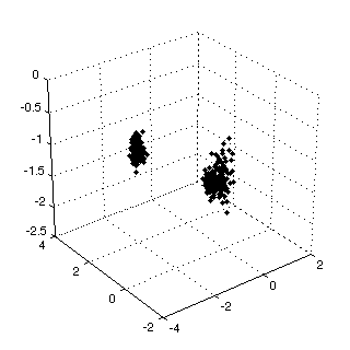 |
Figure 2: PCA initialization of the 3D SOM 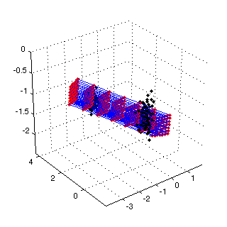 |
Figure 3: trained SOM (input space) 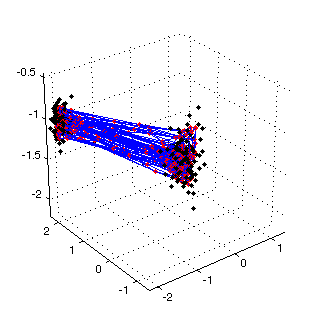 |
Figure 4: trained SOM in the input space and projections in the visualization space 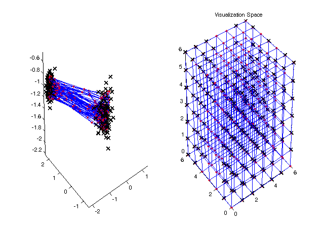 |
Figure 5: SOM component planes 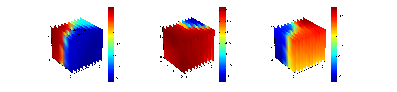 |
Figure 6: 3D distance map (u-matrix) and two activation maps 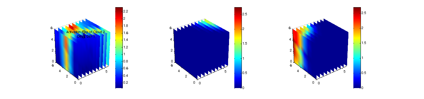 |
Figure 7: projected points in the 3D visualization space 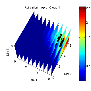 |
|