UniOviSOM grnn regression example

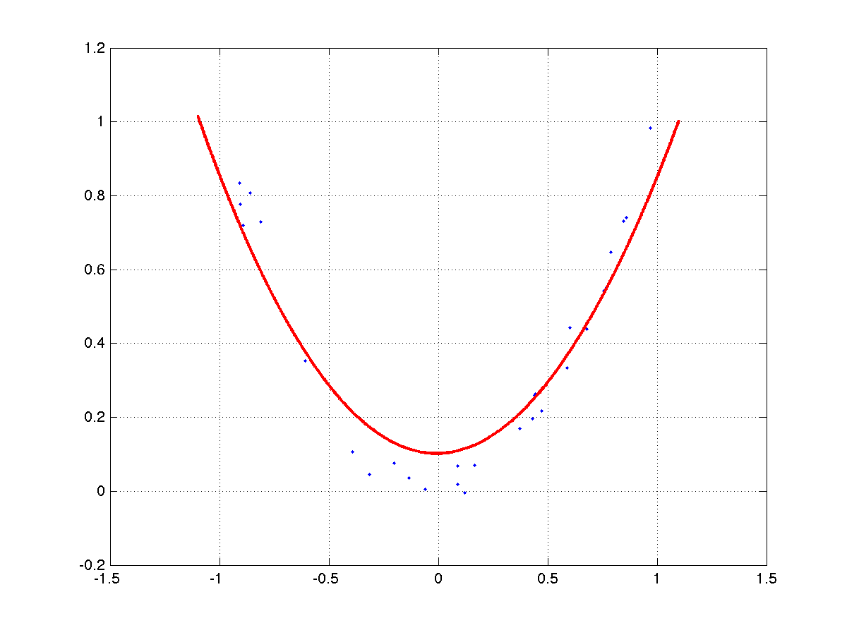
UniOviSOM has several functions to implement regression in an easy way. This example shows how to do 1D interpolation in an easy way. In its basic form, grnntra() trains a generalized regression neural network (GRNN), that can be seen as a normalized rbf (see Specht 1991) that considers normalized rbf's

Donald F. Specht, "A General Regression Neural Network". ''IEEE Transactions on Neural Networks''. 2(6): 568--576. Noviembre, 1991.


figure(1);
clf;

% Create 30 sample points according to a known nonlinear model
N  = 30;
xi = rands(1,N);
yi = xi.^2 + 0.05*randn(1,N);

% plot the points
plot(xi,yi,'.');
grid on;

% width factor
sigma = 10.0;

% train the grnn model (use LS to compute weights)
grnn = grnntra(yi,xi,sigma,1e-6);

% test the model on the interval [-1.1,1.1]
x = linspace(-1.1,1.1,1000);

% predict the y-value using the trained model
yestim = grnnsim(x,grnn);

% plot the results 
hold on;
plot(x,yestim,'r','linewidth',2);
grid on;
hold off;

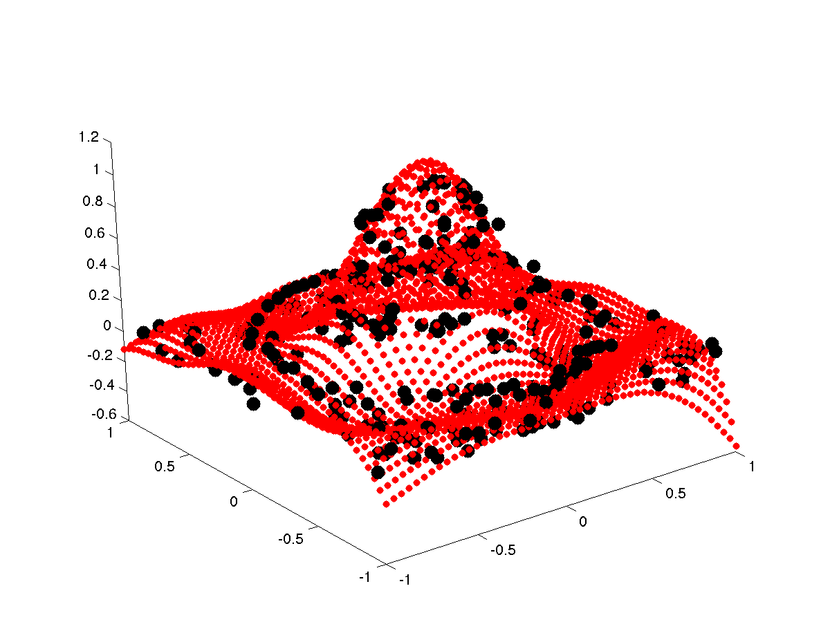
2D regression example

The next example shows a basic 2D regression problem. We take a set of 2D points along with their elevations, and use grnntra/grnnsim to estimate a continuous function z=f(x,y) that approximates the points (see figure).


figure(1);
clf;

clf;
close all;

% create 300 2D points
xi = rands(2,300);

% compute the elevation according to a known nonlinear model
yi = sinc(4*(xi(1,:).^2+xi(2,:).^2));

% plot the resulting 3D points
figure(1);
clf;
plotp([xi;yi],'k.',30);

% test on a square interval on the 2D domain using a regular grid
u = rectop(linspace(-1,1,50),linspace(-1,1,50),'idx');

% width factor
sigma = 0.5;

% train the model
grnn = grnntra(yi,xi,sigma,1e-7);

% predict the elevation using the trained model
yest = grnnsim(u,grnn);

% plot the results (use rotate 3D in the figure to see this better)
hold on;
plotp([u;yest],'r.');
axis([-1,1,-1,1]);
hold off;

Finally, note that there are options in grnntra() to consider least squares estimation of the weights as well as to compute independent terms (see help grnntra() for details).